install.packages(c("RCurl", "jsonlite"))Automated Machine Learning
Introduction
Artificial intelligence (AI), which reaches into many aspects of everyday life, has been extensively explored in recent years. It attempts to use computational devices to automate tasks by allowing them to perceive the environment as humans do. As branch of AI, Machine Learning (ML) enables a computer to perform a task through self-exploration of data. It allows the computer to learn, so it can do things that go beyond what we know how to order it to do. But the barriers to entry are high: the cost of learning the techniques involved and accumulating the necessary experience with applications means practitioners without much expertise cannot easily use ML. Translating ML techniques from theoretical frameworks into practical applications for a broader audience is increasingly a central focus of research and industry. Consequently, autoML has become a prominent area of research. Its objective is to replicate the methodologies employed by human specialists in resolving machine learning challenges and to autonomously identify the most effective machine learning solutions for specific problems, thereby providing practitioners with limited expertise access to readily available machine learning techniques.
In addition to assisting novices, AutoML will alleviate the responsibilities of specialists and data scientists in the creation and configuration of machine learning models. This cutting-edge topic is unfamiliar to many, and its present capabilities are frequently overstated by the media.
What is Machine learning
Machine learning is a subset of artificial intelligence that focuses on building systems that can learn from and make decisions based on data. Unlike traditional programming, where explicit instructions are given, ML algorithms identify patterns and relationship within data to make predictions or decisions. This capability has revolusionised various industries, from healthcare and finance to marketing and transportation.
For example, suppose you want a machine to recognise images of apples and bananas automatically. With symbolic AI, you would need to provide human-readable rules associated with the reasoning process, perhaps specifying features like colour and shape, to the AI method. In contrast, an ML algorithm takes a bunch of images and their corresponding lables (“banana” or “apple”) and outputs the learned rules, which can be used to predict unlabeled images (figure 1).
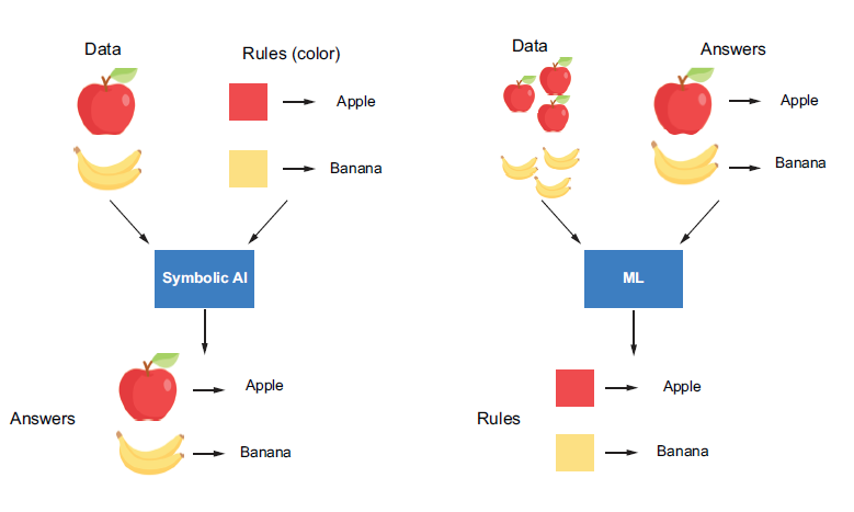
The essential goals of ML are automation and generalization. Automation means an ML algorithm is trained on the data provided to automatically extract rules (or patterns) from the data. It mimics human thinking and allows the machine to improve itself by interacting with the historical data fed to it, which we can training or learning. The rules are then used to perform repetitive predictions on new data without human intervention.
In Figure 1, the ML algorithm interacts with the apple and banana images provided and extracts a colour rule the enables it to recognise them through the training process. These rules can help the machine classify new images without human supervision, which we can generalising to new data. The ability to generalise is an important criterion in evaluating whether an ML algorithm is good. In this case, suppose an image of a yellow apple is fed to the ML algorithm - the colour rule will not enable it to correctly discern whether it’s an apple or a banana. An ML algorithm that learns and applies a shape feature for prediction may provide better predictions.
The Machine Learning Process
An ML algorithm learns rules through exposure to examples with known outputs. The rules are expected to enable it to transform inputs into meaningful outputs, such as transforming images of handwritten digits to the corresponding numbers. So, the goal of learning can also be thought of as enabling data transformation. The learning process generally requires the following two components:
Data inputs- Data instances of the target task to be fed into the ML algorithm, for example, in the image recognition problem (above figure), a set of apple and banana images and their correspoding labels.Learning algorithm- A mathematical procedure to derive a model based on the data inputs, which contains the following 4 elements:- An ML model with a set of
hyperparametersto be learned from the data. - A A
measurementto measure the model’s performance (such as prediction accuracy) with the current hyperparameters. - A way to update the model, which we call an
optimization method. - A
stop criterionto determine when the learning process should stop.
- An ML model with a set of
After the model hyperparameter are intialized, the training algorithm can update the model iteratively by modifying the hyperparameter based on the measurement until the stop criterion is reached. This measurement is called a loss function (or objective function) in the training phase, it measures the difference between the model’s predictions and the ground-truth targets. This process can be illustrated in Figure 2 below:
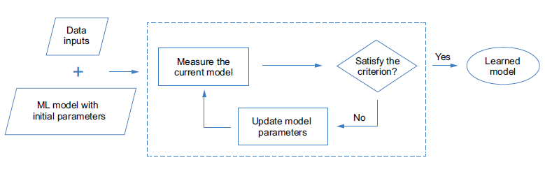 Figure 2: The process of training an ML model
Let’s look at an example to help understand the learning process. Imagine we have a bunch of data points in two-dimensional space (Figure 3). Each point is either black or white. We want to build an ML model that, whenever a new point arrives, can decide whether this is a black point or a white point based on the point’s position. A straightforward way to achieve this goal is to draw a horizontal line to separate the two-dimensional space into two parts based on the data points in hand. This line could be regarded as an ML model. Its parameter is the horizontal position, which can be updated and learned from the provided data points. Coupled with the learning process introduced in Figure 3, the required components could be chosen and summarised as follows:
- The data inputs are a bunch of white and black points described by their location in the two-dimensional space.
- The learning algorithm consists of the following 4 selected components:
- ML model - A horizontal line that can be formulated as \(y=a\), where \(a\) is the parameter that can be updated by the algorithm.
- Accuracy measurement - The percentage of points that are labeled correctly based on the model.
- Optimization method - Move the line up or down by a certain distance. The distance can be related to the value of the measurement in each iteration. It will not stop until the stop criterion is satisfied.
- Stop criterion - Stop when the measurement is 100%, which means all the points in hand are labeled correctly based on the current line.
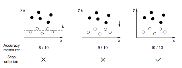
In the example shown in Figure 3, the learning algorithm takes two iterations to achieve the desired line, which separates all the input points correctly. But in practice, this criterion may not always be satisfied. It depends on the distribution of the input data, the selection model type, and how the model is measured and updated. We often need to choose different components and try different combinations to adjust the learning process to get the expected ML solution. Also, even if the learned model is able to label all the training inputs correctly, it is not guaranteed to work well on unseen data. In other words, the model’s ability to generalise may not be good. It’s important to select the components and adjust the learning process carefully.
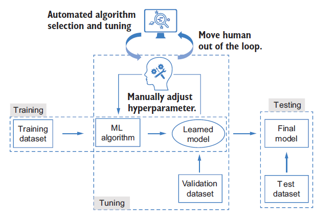
Hyperparameter tuning
How do we select the proper components to adjust the learning process so that we can derive the expected model? To answer this question, we need to introduce a concept called hyperparameters and clarify the relationship between these and the parameters as follows:
Parametersare variables that can be updated by the ML algorithm during the learning proces. They are used to capture the rules from the data. For example, the position of the horizontal line is the only parameter in our previous example (Figure 3) to help classify the points. It is adjusted during the training process by the optimisation method to capture the position rule for splitting the points with different colours. By adjusting the parameters, we can derive an ML model that can accurately predict the outputs of the given input data.Hyperparametersare also parameters, but they are ones we predefine for the algorithm before the learning process begins, and their values remain fixed during the learning process. These include the measurement, the optimisation method, the speed of learning, the stop criterion, and so on. An ML algorithm usually has multiple hyperparameters. Different combinations of them have different effects on the learning process, resulting in ML models with different performances. We can also consider the algorithm type (or the ML model type) as a hyperparameter, because we select it ourselves, and it is fixed during the learning process.
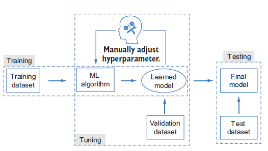
The selection of an optimal combination of hyperparameters for an ML algorithm is callled hyperparameter tuning and is often done through an iterative process. In each iteration, we select a set of hyperparameters to use to learn an ML model with the training dataset. The ML algorithm block in Figure 4 denotes the learning process described in the Figure 2. By evaluating each learned model on a separate dataset called the validation set, we can then pick the best one as the final model. We can evaluate the generalizability of that model using another dataset called the test set, which concludes the whole ML workflow.
In general, we will have three datasets in the ML workflow. Each dataset is distinct from the other two:
- The training set is used during the learning process to train a model given a fixed combination of hyperparameters.
- The validation set is used during the tuning process to evaluate the trained models to select the best hyperparameters.
- The test set is used for the final testing, after the tuning process. It is used only once, after the final model is selected, and should not be used for training or tuning the ML algorithm.
The training and test sets are straightforward to understand. The reason we want to have an additional validation dataset it to avoid exposing the algorithm to all the training data during the tuning stages, - this enhances the generalizability of the final model to unseen data.
This situation will likely lead to bad performance on the final test set, which contains different data. When the model performs worse on the test set (or validation set) than the training set, this is called overfitting. It’s a well-known problem in ML and often happens when the model’s learning capacity is too strong and the size of the training dataset is limited. For example, suppose we want to predict the fourth number of a series, given the first three numbers as training data: \(a_1=1\), \(a_2=2\), \(a_3=3\), \(a_4=?\) ( \(a_4\) is the validation set here, \(a_5\) onward are the test sets.) If the right solution is \(a_4=4\), a naive model, \(a_i\), would provide the correct answer. If you use a third-degree polynomial to fit the series, a perfect solution for the training data would be \(a_i=i3 - 6i^2 + 12i - 6\), which will predict \(a_4\) as 10. The validation process enables a model’s generalization ability to be better reflected during evaluation that better models can be selected.
Note
Overfitting is one of the most important problems studied in ML. Besides doing validation during the tuning process, we have many other ways to address the problem, such as augmenting the dataset, adding regularization to the model to contrain its learning capacity during training, and so on.
The obstacles to applying machine learning
At this point, we have some basic understanding of what ML is and how it proceeds. Although we can make use of many mature ML toolkits, we may still face difficulties in practice. Some challenges in applying machine learning are:
- The cost of learning ML techniques - so far, we have covered some basics, but more knowledge is required when applying ML to a real problem. For example, we need to think about how to formulate problem as an ML problem, which ML algorithms we could use for our problem and how they work, how to clean and preprocess the data into the expected format to input into our ML algorithm, which evaluation criteria should be selected for model training and hyperparameter tuning, and so on. All these questions need to be answered in advance, and doing so may require a large time commitment.
- Implementation complexity - Even with the necessary knowledge and experience implementing the workflow after selecting an ML algorithm is a complex task. The time required for implementation and debugging will grow as more advanced algorithms are adopted.
- The gap between theory and practice - The learning process can be hard to interpret, and the performance is highly data driven. Furthermore, the datasets used in ML are often complex and noisy and can be defficult to interpret, clean, and control. This means the tuning process is often more empirical than analytical. Even ML experts sometimes cannot achieve the desired results.
These difficulties significantly impede the democratisation of ML to people with limited experience and correspondingly increase the burden on ML experts. This has motivate ML researchers and practitioners to pursue a solution to lower the barriers, circumvent the unnecessary procedures, and alleviate the burden of manual algorithm design and tuning - AutoML.
Importance of Automation in ML
The process of developing ML models involves several steps, including data preprocessing, feature selection, model training, and evaluation. Each of these steps can be time-consuming and requires significant expertise. Automation in ML, often referred to as Automated Machine Learning (AutoML), aims to streamline these processes, making it easier and faster to develop high-performing models. By automating repetitive and complex tasks, AutoML allows data scientist and analysts to focus on more strategic aspects of their work.
Introduction to AutoML and Its Benefits AutoML refers to the use of automated tools and techniques to perform various stages of the ML pipeline. These tools can automatically preprocess data, select features, train multiple models, and evaluate their performance to identify the best one. The benefits of AutoML include:
Efficiency: Reduces the time and effort required to build ML models.
Accessibility: Makes ML accessible to non-experts by simplifying the model-building process.
Performance: Often results in models that are as good as or better than those built manually by experts.
Scalability: Enables the development of multiple models simultaneously, which is particularly useful for large-scale projects.
AutoML
AutoML is the process of automating the various steps that are performed while developing a viable ML system for predictions. A typical ML pipeline consists of the following steps:
Data collection:This is the very first step in an ML pipeline. Data is collected from various sources. The sources can generate different types of data, such as categorical, numeric, textual, time series, or even visual and auditory data. All these types of data are aggregated together based on the requirements and are merged into a common structure. This could be a comma-separated value file, a parquet file, or even a table from a database.Data exploration:Once data has been collected, it is explored using basic analytical techniques to identify what is contains, the completeness and correctness of the data, and if the data shows potential patterns that can build a model.Data preparation:Missing values, duplicates, and noisy data can all affect the quality of the model as they introduce incorrect learning. Hence, the raw data that is collected and explored needs to be pre-processed to remove all anomalies using specific data processing methods.Data transformation:A lot of ML models work with different types of data. Some can work with categorical data, while some can only work with numeric data. That is why you may need to convert certain types of data from on form into the other. This allows the dataset to be fed properly during model training.Model selection:Once the dataset is ready, an ML model is selected to be trained. The model is chosen based on what type of data the dataset contains, what information is to be extracted from the dataset, as well as which model suits the data.Model training:This is where the model is trained. The ML system will learn from the processed dataset and create a model. This training can be influenced by several factors, such as data attribute weighting, learning rate, and other hyperparameters.Hyperparameter tuning:Apart from model training, another factor that need to be considered is the model’s architecture. The model’s architecture depends on the type of algorithm used, such as the number of trees in a random forest or neurons in a neural network. We don’t immediately know which architecture is optimal for a given model, so experimentation is needed. The parameters that define the architecture of a model are called hyperparameters, finding the best combination of hyperparameter values is known as hyperparameter tuning.Prediction:The final step of the ML pipeline is prediction. Based on the patterns in the dataset that were learned by the model during training, the model can now make a generalised prediction on unseen data.
For non-experts, all these steps and their complexities can be overwhelming. Every step in the ML pipeline process has been developed over years of research and there are vast topics within themselves. AutoML is the process that automates the majority of these steps, from data exploration to hyperparameter tuning, and provides the best possible models to make prediction on. This helps companies focus on solving real-world problems with results rather than ML processes and workflows.
AutoML: The Automation of Automation
The goal of AutoML is to allow a machine to mimic how humans design, tune, and apply ML algorithms so that we can adopt ML more easily (Figure 5). Because a key property of ML is automation, AutoML can be regarded as automating automation.
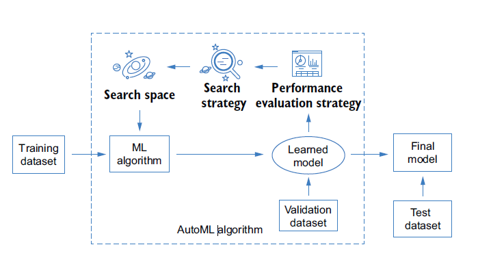
Each AutoML algorithm consists of the following three core components (Figure 6):
- Search space - a set of hyperparameters, and the ranges of each hyperparameter from which to select. The range of each hyperparameter can be defined based on the user’s requirements and knowledge. For example, the search space can be a pool of ML algorithms. In this case, we treat the type of ML algorithm as a hyperparameter to be selected. The search space can also be the hyperparameters of a specific ML algorithm, such as the structure of the ML model. The design of the search space is highly task-dependent, because we may need to adopt different ML algorithms for various tasks. It is also quite personalised and ad hoc, depending on the user’s interests, expertise, and level of experience. There is always a tradeoff between the convenience we will enjoy by defining a large search space and the time we spend identifying a good model (or the performance of the model we can achieve in a limited amount of time). For beginners, it can be tempting to define a broad search space that is genral enough to apply to any task or situation, such as search space containing all the ML algorithms - but the time and computational cost involved make this a poor solution.
- Search Strategy - a strategy to select the optimal set of hyperparameters from the search space. Because AutoML is often an iterative trial-and-error process, the strategy often sequentially selects the hyperparameters in the search space and evaluates their performance. It may loop through all the hyperparameters in the search space, or the search strategy may be adapted based on the hyperparameters that have been evaluated so far to increase the efficiency of the later trials. A better search strategy can help us to achieve a better ML solution within the same amount of time. It may also allow us to use a larger search space by reducing the search time and computational cost.
- Performance evaluation strategy - A way to evaluate the performance of a specific ML algorithm instantiated by the selected hyperparameters. The evaluation criteria are often the same as the ones used in manual tuning, such as the validation performance of the model learned from the selected ML algorithm.
Why use AutoML?
Challenges in Traditional ML Model Building Building ML models traditionally involves several challenges:
Time-Consuming: The process of data cleaning, feature engineering, model selection, and hyperparameter tuning can be very time-consuming.
Resource-Intensive: Requires significant computational resources and expertise.
Complexity: Managing and optimizing multiple models and parameters can be complex and error-prone.
Time and Resource Efficiency AutoML addresses these challenges by automating many of the labor-intensive tasks involved in model building. This leads to significant time savings and allows data scientists to focus on higher-level tasks. Additionally, AutoML tools often come with built-in optimization techniques that ensure efficient use of computational resources.
Improved Accuracy and Performance AutoML tools leverage advanced algorithms and techniques to explore a wide range of models and hyperparameters. This often results in models that are more accurate and perform better than those developed manually. By systematically evaluating multiple models, AutoML ensures that the best possible model is selected for a given task.
Democratizing ML for Non-Experts One of the most significant benefits of AutoML is its ability to democratize ML. By simplifying the model-building process, AutoML makes it accessible to individuals who may not have extensive expertise in ML. This opens up opportunities for a broader range of professionals to leverage ML in their work, fostering innovation and enabling data-driven decision-making across various fields.
Overview of AutoML in R
Introduction to R and Its Ecosystem for ML R is a powerful programming language and environment widely used for statistical computing and data analysis. It has a rich ecosystem of packages and tools that make it an excellent choice for machine learning (ML) tasks. R’s extensive libraries, such as caret, mlr3, and h2o, provide robust functionalities for data preprocessing, model training, and evaluation.
Key AutoML Packages in R Several packages in R are designed to facilitate AutoML, each offering unique features and capabilities:
h2o: One of the most popular AutoML packages,h2oprovides a comprehensive suite of tools for building and deploying ML models. It supports a wide range of algorithms and offers automated model selection and hyperparameter tuning.caret: Thecaretpackage (short for Classification and Regression Training) streamlines the process of creating predictive models. It includes functions for data splitting, pre-processing, feature selection, and model tuning using resampling.mlr3: Themlr3package is a modern, flexible, and extensible framework for ML in R. It supports a wide variety of ML algorithms and provides tools for automated hyperparameter tuning, model evaluation, and benchmarking.autoML: This package focuses on simplifying the ML workflow by automating the selection and tuning of models. It is designed to be user-friendly and integrates well with other R packages.
Basic Workflow of an AutoML Process The typical workflow of an AutoML process in R involves several key steps:
Data Preparation: Load and preprocess the data, including handling missing values, encoding categorical variables, and normalizing numerical features.
Model Training: Use an AutoML package to train multiple models on the prepared data. The package will automatically select the best algorithms and tune their hyperparameters.
Model Evaluation: Evaluate the performance of the trained models using appropriate metrics (e.g., accuracy, precision, recall). The AutoML package will typically provide a leaderboard of models ranked by their performance.
Model Selection: Choose the best-performing model based on the evaluation metrics. The selected model can then be used for making predictions on new data.
Deployment: Deploy the selected model for use in a production environment. This may involve saving the model to disk, integrating it into a web service, or using it within a larger data pipeline.
H2O AutoML
H2O AutoML developed by H2O.ai that simplifies how ML systems are developed by providing user-friendly interfaces that help non-experts experiment with ML. It is an in-memory, distributed, fast and scalable ML and analytics platform that works on big data and can be used for enterprise needs.
It is written in Java and uses key-value storage to access data, models, and other ML objects that are involved. It runs on a cluster system and uses the multi-threaded MapReduce framework to parallelize data operations. It is also easy to communicate with it as it uses simple REST APIs. Finally, it has a web interface that provides a detailed graphical view of data and model details.
Not only does H2O AutoML automate the majority of the sophosticated steps involved in the ML life cycle, but it also provides a lot of flexibility for even expert data scientist to implement specialized model training processes. H2O AutoML provides a simple wrapper functions that encapsulates several of the model training tasks that would otherwise be complicated to orcestrate. It also has extensive explainability functions that can describe the various details of the model training life cycle. This provides easy-to-export details of the models that users can use to explain the performance and justifications of the models that have beedn trained.
The best part about H2O AutoML is that it is entirely open source. We can find H2O’s source code at https://github.com/h2oai. It is actively maintained by a community of developers serving in both open as well as closed sources companies. At the time of writing, it is on its third major version, which indicates that it is quite a mature technology and is feature-intensive – that is, it supports several major companies in the world. It also supports several programming languages, including R, Scala, Python, and Java, that can run on several operating systems and provides support for a wide variety of data sources that are involved in the ML life cycle, such as Hadoop Distributed File System, Hive, Amazon S3, and even Java Database Connectivity (JDBC).
Minimum System Requirement to use H2O AutoML
Hardware:
- Memory - H2O runs on an in-memory architecture, so it is limited by the physical memory of the system that uses it. Thus, to be able to process huge chucks of data, the more memory the system, has the better.
- Central Processing Unit (CPU) - by default, H2o will use the maximum available CPUs of the system. However, at a minimum, it will need 4 CPUs.
- Graphical Processing Unit (GPU) - GPU support is only available for XGBoost models in AutoML if the GPUs are NVIDIA GPUs (GPU Cloud, DGX Station, DGX-1, or DGX-2) or if it is a CUDA 8 GPU.
- The operating systems that support H2O are as follows:
- Ubuntu 12.04
- OS X 10.9 or later
- Windows 7 or later
- CentOS 6 or later
- The programming languages that support H2O are as follows:
- Java - Java is mandatory for H2O. H2O requires a 64-bit JDK to build H2O and a 64-bit JRE to run its binary:
- Java version supported: Java SE 15, 14, 13, 12, 11, 10, 9, and 8
- Other languages -
- Python 2.7x, 3.5x, or later
- Scala 2.10 or later
- R version 3 or later
- Java - Java is mandatory for H2O. H2O requires a 64-bit JDK to build H2O and a 64-bit JRE to run its binary:
- Additional requirements - The following requirements are only needed if H2O is being run in these environments:
- Hadoop - Cloudera CDH 5.4 or later, Hortonworkds HDP 2.2 or later, MapR 4.0 or later or IBM Open Platform 4.2
- Conda - 2.7, 3.5, or 3.6
- Spark - Version 2.1, 2.2, or 2.3
Installing Java
H2O’s core code is written in Java. It needs Java Runtime Environment (JRE) installed in our system to spin up an H2O server cluster. H2O also trains all the ML algorithms in a multi-threaded manner, which uses the Java Fork/Join framework on top of its MapReduce framework. Hence, having the latest Java version that is compatible with H2O to run H2O smoothly is highly recommended.
To install latest stable of Java
https://www.oracle.com/java/technologies/downloads/
When installing Java, it is important to be aware of which bit version your system runs on. If it is a 64-bit verison, then make sure you are installing the 64-bit Java version for your operating system. If it is 32-bit, then go for the 32-bit version.
Installing H2O in R
To install the R packages, follow these steps:
- First, we need to download the H2O R package dependencies. For this, execute the following command in R Terminal.
- Then, depending on internet connection, please increase the download time since the H2O package is too large.
options(timeout = 600)
#this would increase time to download the package to 600 seconds, by default is 60 seconds- Install the actual
h2opackage, execute the following command in the R console.
install.packages("h2o")or, you can download the latest version of h2o package from the website via this link: http://h2o-release.s3.amazonaws.com/h2o/latest_stable.html. As to date (23rd October 2024), the latest version is 3.46.0.5. Please refer to this page to download this version.
# The following two commands remove any previously installed H2O packages for R.
if ("package:h2o" %in% search()) { detach("package:h2o", unload=TRUE) }
if ("h2o" %in% rownames(installed.packages())) { remove.packages("h2o") }

# Next, we download packages that H2O depends on.
pkgs <- c("RCurl","jsonlite")
for (pkg in pkgs) {
if (! (pkg %in% rownames(installed.packages()))) { install.packages(pkg) }
}

# Now we download, install and initialize the H2O package for R.
install.packages("h2o", type="source", repos="https://h2o-release.s3.amazonaws.com/h2o/rel-3.46.0/5/R")

# Finally, let's load H2O and start up an H2O cluster
library(h2o)
h2o.init()- To test if it has been successfully downloaded and installed, import the library and execute the
h2o.init()command. This will spin up a local H2O server.
#calling the library
library(h2o)

#Initiate the server
h2o.init()
After executing h2o.init(), the H2O client will check if there is an H2O server instance already running on the system. The H2O server is usually run locally on port 54321 by default. If it had found an already existing local H2O instance on the port, then it would have reused the same instance. However, in this scenario, there wasn’t any H2O server instance running on port 54321, which is why H2O attempted to start a local server on the same port.
Next, you will see the location of the JVM logs. Once the server is up and running, the H2O client tries to connect to it and the status of the connection to the server is displayed. Lastly you will see some basic metadata regarding the server’s configuration. This metadata may be slightly different from what you see in your execution as it depends a lot on the specifications of your system.
For example, by default, H2O will use all the cores available on your system for processing. So, if you have an 8-core system, then the H2O_cluster_allowed_cores property value will be 8. Alternatively, if you decide to use only four cores, then you can execute the h2o.init(nthreads=4) command to use only four cores, thus reflecting the same in the server configuration output.
Training our first ML model using H2O AutoML
All ML pipelines, whether they are automated or not, eventually follow the same ML workflows discussed earlier.
Understanding the GSE140829 dataset
The GSE140829 dataset’s series matrix file is retrieved from the GEO database using the following search terms: “Alzheimer’s disease,” “inflammation,” “homo sapiens,” and “expression profiling by an array. This dataset was generated using the GPL15988 HumanHT-12 v4 expression. Download the dataset here.
This dataset consists 17 biomarkers that already validated from Literature and 1 target variable. There are 249 Control subjects and 204 AD patients in the dataset.
The following is first 10 observations in the dataset:
data1 <- read.csv("GSE140829.csv")
data1$Group <- as.factor(data1$Group)

table(data1$Group)
     AD Control
    204     249
Model Training
Model training is the process of finding the best combination of biases and weights for a given ML algorithm so that it minimizes a loss function. A loss function is a way of measuring how far the predicted value is from the actual value. So, minimizing it indicates that the model is getting closer to making accurate predictions.
The ML algorithm builds a mathematical representation of the relationship between the various variables in the dataset and the target label. Then, we use this mathematical representation to predict the potential value of the target label for certain variable values. The accuracy of the predicted values depend a lot on the quality of the dataset, as well as the combination of weights and biases against variables used during model training. However, all of this is entirely automated by AutoML and, as such, is not a concern for us.
Model training and prediction in R
Follow these steps:
- Import the H2O library
library(h2o)Warning: package 'h2o' was built under R version 4.4.1- Initialize H2O to spin up a local H2O server
h2o.init() Connection successful!
R is connected to the H2O cluster:
H2O cluster uptime: 24 minutes 7 seconds
H2O cluster timezone: Asia/Singapore
H2O data parsing timezone: UTC
H2O cluster version: 3.44.0.3
H2O cluster version age: 10 months and 4 days
H2O cluster name: H2O_started_from_R_USER_lur034
H2O cluster total nodes: 1
H2O cluster total memory: 3.88 GB
H2O cluster total cores: 8
H2O cluster allowed cores: 8
H2O cluster healthy: TRUE
H2O Connection ip: localhost
H2O Connection port: 54321
H2O Connection proxy: NA
H2O Internal Security: FALSE
R Version: R version 4.4.0 (2024-04-24 ucrt) Warning in h2o.clusterInfo():
Your H2O cluster version is (10 months and 4 days) old. There may be a newer version available.
Please download and install the latest version from: https://h2o-release.s3.amazonaws.com/h2o/latest_stable.htmlh2o.init() will start up an H2O server instance that’s running locally on port 54321 and connect to it. If an H2O server already exists on the same port, then it will reuse it.
- Import the dataset using
h2o.importFile()by passing the location where you downloaded the dataset. Import the dataset:
data1 <- h2o.importFile("GSE140829.csv")since we already import data1 in R environment, we straight away call the dataset as data1
data1 <- as.h2o(data1)
  |
  |                                                                      |   0%
  |
|======================================================================| 100%- Now, we need to set which columns of the dataframe are the variables and which column is the label. We will set
Speciesas the target label and the remaining column names as the list of the variables:
y<- "Group"
x <- setdiff(names(data1), y)- Split the dataframe into two parts, One part of the data will be used for training, while the other will be used for testing/validating the model being trained.
parts <- h2o.splitFrame(data1, 0.7, seed=1234)splits the dataframe into two parts. One part contains 70% of the data, while the other contains the remaining 30%.
parts <- h2o.splitFrame(data1, 0.7, seed = 1234)Now, assign the dataframe that contains 70% of the data as the training set and the other as the testing or validation set.
- Assign the first part as the training set
train <- parts[[1]]- Assign the second part as the testing set
test <- parts[[2]]- For classification problem, the response variable should be a factor level.
train[ , y] <- as.factor(train[ , y])
test[ , y] <- as.factor(test[ , y])
Now, the dataset has been imported and its variables and labels have been identified, Let’s pass them to H2O’s AutoML to train models.
This means that we can implement the AutoML model training function in R using h2o.automl(). To understand the function usage, we can always look at the documentation using ?h2o.automl().
The AutoML makes findings the best (or almost best) model extremely fast and easy, because it is all combined in a single function, that only needs a dataset, the target in case of classification and a time or model number limit that tells it how long to train model for. AutoML trains a number of different algorithms during a default classification run in this specific orders:
- 1 Generalized Linear Model (GLM)
- 1 Distributed Random Forest (DRF)
- 1 Extremely Randomized Trees (XRT)
- 3 Extreme Gradient Boosting (XGBoost) - only available on GPU
- 1 Gradient Boosting Machine (GBM)
- Deep Learning - a neural net, a random grid of XGBoost, a random grid of GBMs and a random grid of Neural Nets.
- 2 Stacked Ensembles - The 2 ensembles is calculated from all models, the others only from the best model of each family of algorithms.
For all algorithms where multiple models are run, autoML automatically tests a range of hyperparameters for different arguments.
Here the quick example to use the function:
- Train the model using
h2o.automl, Here, we only ask to produce 12 models with minimal time 60 seconds to save memory and time to compile this html file. You can adjust this at your own convenience.
auto1 <- h2o.automl(x = x, #all independent variables
                    y=y,  # the target variable
                    training_frame = train, #using train set
                    max_models = 12, #number of model to produce
                    seed = 123456, # set seed
                    nfold = 10, #k-fold cros-validation
                    max_runtime_secs = 60, #setting max run time in second
                    )
  |
  |                                                                      |   0%
  |
  |====                                                                  |   6%
18:01:23.191: AutoML: XGBoost is not available; skipping it.
  |
  |============                                                          |  18%
  |
  |===============================                                       |  44%
  |
  |=================================                                     |  47%
  |
  |======================================                                |  55%
  |
  |==========================================                            |  59%
  |
  |=============================================                         |  64%
  |
  |================================================                      |  69%
  |
  |======================================================================| 100%
#Other arguments that can be imputed
#stopping_metric = "AUTO", #by default AUTO is logloss for classification and deviance for regression
#distribution = "AUTO" #Automatic detect the distribution of the data
#balance_classes = TRUE, #this is for balance grouph2o AutoML produce a leaderboard to show all the models performed. It returns all models that ranked by the choose metrics. In our example, the stopping_metric use is “AUTO” by default. We can choose stopping metric as follows: c("AUTO", "deviance", "logloss", "MSE", "RMSE", "MAE", "RMSLE", "AUC", "AUCPR", "lift_top_group", "misclassification", "mean_per_class_error").
- Extract the AutoML Leaderboard
model_leaderboard <- auto1@leaderboard- To display the AutoML leaderboard, we can use the print function, this will display top 6 models. If you wanted to display all models that have been performed, just type
as.data.frame(auto1@leaderboard).
print(model_leaderboard[, c(1,2,3)]) model_id auc logloss
1 GBM_grid_1_AutoML_2_20241024_180123_model_1 0.7318403 0.6049244
2 XRT_1_AutoML_2_20241024_180123 0.7298750 0.6185802
3 StackedEnsemble_BestOfFamily_1_AutoML_2_20241024_180123 0.7283177 0.6125810
4 GBM_grid_1_AutoML_2_20241024_180123_model_2 0.7275390 0.6098285
5 GLM_1_AutoML_2_20241024_180123 0.7265750 0.6184231
6 DRF_1_AutoML_2_20241024_180123 0.7199748 0.6214645
[14 rows x 3 columns] Once the training has finished, AutoML will create a leaderboard of all the models it has trained, ranking them from the best performing to the worst.
- To display the best model in the analysis
best_model <- h2o.get_best_model(auto1)
print(best_model)
Model Details:
==============
H2OBinomialModel: gbm
Model ID: GBM_grid_1_AutoML_2_20241024_180123_model_1
Model Summary:
number_of_trees number_of_internal_trees model_size_in_bytes min_depth
1 27 27 3311 2
max_depth mean_depth min_leaves max_leaves mean_leaves
1 5 3.44444 4 6 5.11111
H2OBinomialMetrics: gbm
** Reported on training data. **
MSE: 0.1632561
RMSE: 0.4040496
LogLoss: 0.5056833
Mean Per-Class Error: 0.2269828
AUC: 0.8750417
AUCPR: 0.8927156
Gini: 0.7500834
R^2: 0.3407768
Confusion Matrix (vertical: actual; across: predicted) for F1-optimal threshold:
AD Control Error Rate
AD 97 52 0.348993 =52/149
Control 19 162 0.104972 =19/181
Totals 116 214 0.215152 =71/330
Maximum Metrics: Maximum metrics at their respective thresholds
metric threshold value idx
1 max f1 0.451561 0.820253 212
2 max f2 0.355831 0.894309 258
3 max f0point5 0.591547 0.852660 136
4 max accuracy 0.566837 0.806061 157
5 max precision 0.865250 1.000000 0
6 max recall 0.208638 1.000000 318
7 max specificity 0.865250 1.000000 0
8 max absolute_mcc 0.566837 0.618972 157
9 max min_per_class_accuracy 0.542825 0.791946 173
10 max mean_per_class_accuracy 0.566837 0.810746 157
11 max tns 0.865250 149.000000 0
12 max fns 0.865250 179.000000 0
13 max fps 0.144817 149.000000 328
14 max tps 0.208638 181.000000 318
15 max tnr 0.865250 1.000000 0
16 max fnr 0.865250 0.988950 0
17 max fpr 0.144817 1.000000 328
18 max tpr 0.208638 1.000000 318
Gains/Lift Table: Extract with `h2o.gainsLift(<model>, <data>)` or `h2o.gainsLift(<model>, valid=<T/F>, xval=<T/F>)`
H2OBinomialMetrics: gbm
** Reported on cross-validation data. **
** 10-fold cross-validation on training data (Metrics computed for combined holdout predictions) **
MSE: 0.2089831
RMSE: 0.4571467
LogLoss: 0.6049244
Mean Per-Class Error: 0.3566688
AUC: 0.7318403
AUCPR: 0.7737931
Gini: 0.4636805
R^2: 0.1561326
Confusion Matrix (vertical: actual; across: predicted) for F1-optimal threshold:
AD Control Error Rate
AD 60 89 0.597315 =89/149
Control 21 160 0.116022 =21/181
Totals 81 249 0.333333 =110/330
Maximum Metrics: Maximum metrics at their respective thresholds
metric threshold value idx
1 max f1 0.400450 0.744186 248
2 max f2 0.171936 0.860266 327
3 max f0point5 0.645946 0.711893 103
4 max accuracy 0.488262 0.684848 198
5 max precision 0.936149 1.000000 0
6 max recall 0.171936 1.000000 327
7 max specificity 0.936149 1.000000 0
8 max absolute_mcc 0.645946 0.366446 103
9 max min_per_class_accuracy 0.515936 0.657718 170
10 max mean_per_class_accuracy 0.502115 0.676721 187
11 max tns 0.936149 149.000000 0
12 max fns 0.936149 180.000000 0
13 max fps 0.091955 149.000000 329
14 max tps 0.171936 181.000000 327
15 max tnr 0.936149 1.000000 0
16 max fnr 0.936149 0.994475 0
17 max fpr 0.091955 1.000000 329
18 max tpr 0.171936 1.000000 327
Gains/Lift Table: Extract with `h2o.gainsLift(<model>, <data>)` or `h2o.gainsLift(<model>, valid=<T/F>, xval=<T/F>)`
Cross-Validation Metrics Summary:
mean sd cv_1_valid cv_2_valid cv_3_valid
accuracy 0.721212 0.086657 0.727273 0.757576 0.787879
auc 0.729556 0.062705 0.680147 0.775735 0.842308
err 0.278788 0.086657 0.272727 0.242424 0.212121
err_count 9.200000 2.859681 9.000000 8.000000 7.000000
f0point5 0.732710 0.087328 0.700000 0.738636 0.817308
f1 0.770148 0.069351 0.756757 0.764706 0.829268
f2 0.823366 0.092708 0.823529 0.792683 0.841584
lift_top_group 1.497500 0.815038 0.000000 2.062500 1.650000
logloss 0.617345 0.056858 0.692363 0.597780 0.496956
max_per_class_error 0.515404 0.211392 0.411765 0.294118 0.307692
mcc 0.447344 0.135007 0.481267 0.520299 0.550848
mean_per_class_accuracy 0.698119 0.083497 0.731618 0.759191 0.771154
mean_per_class_error 0.301881 0.083497 0.268382 0.240809 0.228846
mse 0.214231 0.023325 0.237587 0.205792 0.165731
pr_auc 0.756926 0.095910 0.565106 0.797458 0.909589
precision 0.715353 0.116591 0.666667 0.722222 0.809524
r2 0.116220 0.088241 0.048778 0.176077 0.305843
recall 0.870530 0.130428 0.875000 0.812500 0.850000
rmse 0.462207 0.025739 0.487429 0.453643 0.407100
specificity 0.525707 0.256983 0.588235 0.705882 0.692308
cv_4_valid cv_5_valid cv_6_valid cv_7_valid cv_8_valid
accuracy 0.757576 0.818182 0.787879 0.575758 0.666667
auc 0.744444 0.785124 0.739669 0.666667 0.629630
err 0.242424 0.181818 0.212121 0.424242 0.333333
err_count 8.000000 6.000000 7.000000 14.000000 11.000000
f0point5 0.784314 0.847458 0.807692 0.616438 0.674603
f1 0.666667 0.869565 0.857143 0.720000 0.755556
f2 0.579710 0.892857 0.913044 0.865385 0.858586
lift_top_group 2.200000 0.000000 1.500000 1.833333 1.833333
logloss 0.624328 0.573857 0.620551 0.645134 0.693704
max_per_class_error 0.466667 0.363636 0.545455 0.933333 0.666667
mcc 0.534172 0.577350 0.500000 0.193649 0.358610
mean_per_class_accuracy 0.738889 0.772727 0.704545 0.533333 0.638889
mean_per_class_error 0.261111 0.227273 0.295455 0.466667 0.361111
mse 0.221084 0.192589 0.216653 0.228252 0.248687
pr_auc 0.787152 0.797473 0.844473 0.740833 0.664009
precision 0.888889 0.833333 0.777778 0.562500 0.629630
r2 0.108295 0.133350 0.025059 0.079385 -0.003038
recall 0.533333 0.909091 0.954545 1.000000 0.944444
rmse 0.470196 0.438850 0.465460 0.477757 0.498685
specificity 0.944444 0.636364 0.454545 0.066667 0.333333
cv_9_valid cv_10_valid
accuracy 0.757576 0.575758
auc 0.729630 0.702206
err 0.242424 0.424242
err_count 8.000000 14.000000
f0point5 0.754717 0.585938
f1 0.800000 0.681818
f2 0.851064 0.815217
lift_top_group 1.833333 2.062500
logloss 0.611177 0.617603
max_per_class_error 0.400000 0.764706
mcc 0.516398 0.240852
mean_per_class_accuracy 0.744444 0.586397
mean_per_class_error 0.255556 0.413603
mse 0.209857 0.216083
pr_auc 0.713605 0.749558
precision 0.727273 0.535714
r2 0.153577 0.134875
recall 0.888889 0.937500
rmse 0.458101 0.464847
specificity 0.600000 0.235294[1] "Our best model id is GBM_grid_1_AutoML_2_20241024_180123_model_1 we can inspect the detail of the best model by using '@' after the best_model"To display the parameters used in the best model:
best_model@parameters$model_id
[1] "GBM_grid_1_AutoML_2_20241024_180123_model_1"
$training_frame
[1] "AutoML_2_20241024_180123_training_RTMP_sid_a8cf_6"
$nfolds
[1] 10
$keep_cross_validation_models
[1] FALSE
$keep_cross_validation_predictions
[1] TRUE
$score_tree_interval
[1] 5
$fold_assignment
[1] "Modulo"
$ntrees
[1] 27
$min_rows
[1] 30
$stopping_metric
[1] "logloss"
$stopping_tolerance
[1] 0.05
$seed
[1] 123456
$distribution
[1] "bernoulli"
$sample_rate
[1] 0.6
$col_sample_rate
[1] 0.7
$col_sample_rate_per_tree
[1] 0.4
$min_split_improvement
[1] 1e-04
$histogram_type
[1] "UniformAdaptive"
$categorical_encoding
[1] "Enum"
$calibration_method
[1] "PlattScaling"
$x
[1] "CDC26" "CTNNBIP1" "DZIP1" "FGGY" "GYG1" "LRPAP1"
[7] "MAPK14" "MOSC1" "MTMR10" "PPAPDC1B" "RDH13" "S100A4"
[13] "SNAI3" "TANC2" "TBKBP1" "TPST1" "ZNF513"
$y
[1] "Group"We can also extract specific model that we think is the best to apply in prediction, for example, Based on the leaderboard, I want to select model no 2, the model id for 2nd best model is: XRT_1_AutoML_2_20241023_144643
auto1@leaderboard[2,][1] model_id
1 XRT_1_AutoML_2_20241024_180123
[1 row x 1 column] To get the model XRT_1_AutoML_2_20241023_144643:
h2o.getModel("XRT_1_AutoML_2_20241023_144643")- To display variable important from best model:
h2o.varimp_plot(best_model)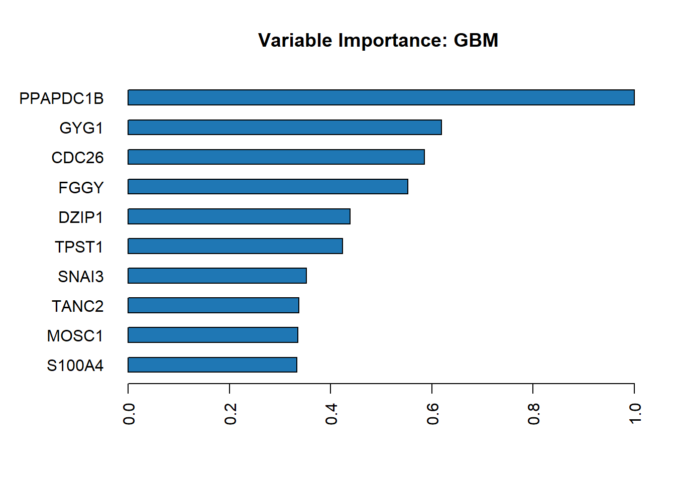
To display the values
h2o.varimp(best_model)Variable Importances:
variable relative_importance scaled_importance percentage
1 PPAPDC1B 22.766836 1.000000 0.159169
2 GYG1 14.083176 0.618583 0.098459
3 CDC26 13.318046 0.584976 0.093110
4 FGGY 12.572194 0.552215 0.087896
5 DZIP1 9.985238 0.438587 0.069809
6 TPST1 9.644176 0.423606 0.067425
7 SNAI3 8.023937 0.352440 0.056098
8 TANC2 7.664796 0.336665 0.053587
9 MOSC1 7.634538 0.335336 0.053375
10 S100A4 7.577775 0.332843 0.052978
11 CTNNBIP1 6.527891 0.286728 0.045638
12 RDH13 6.447965 0.283217 0.045079
13 MAPK14 4.158609 0.182661 0.029074
14 TBKBP1 4.091538 0.179715 0.028605
15 MTMR10 3.543033 0.155623 0.024770
16 LRPAP1 3.006824 0.132070 0.021022
17 ZNF513 1.988951 0.087362 0.013905- To show variable importance from all models
h2o.varimp_heatmap(auto1)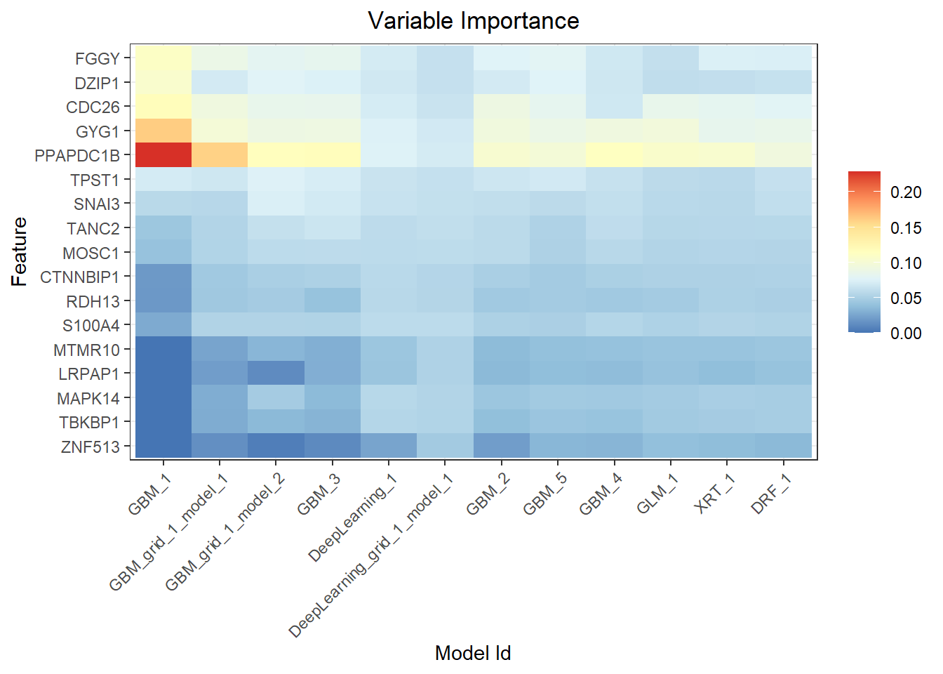
- To make predictions
predictions <- h2o.predict(auto1, test)
  |
  |                                                                      |   0%
  |
|======================================================================| 100%head(predictions) predict AD Control
1 Control 0.3316200 0.6683800
2 Control 0.2831339 0.7168661
3 Control 0.2349890 0.7650110
4 Control 0.1651689 0.8348311
5 Control 0.1898736 0.8101264
6 Control 0.1851188 0.8148812The predict function of the h2o object accepts two parameters. One is the model object, which in our case is the auto1 object, while the other is the dataframe to make predictions on. By default, the auto1 object will use the best model in the leaderboard to make predictions.
similarly, we can straight away use the best model to make prediction
prediction1 <- h2o.predict(best_model, test)
  |
  |                                                                      |   0%
  |
|======================================================================| 100%head(prediction1) predict AD Control
1 Control 0.3316200 0.6683800
2 Control 0.2831339 0.7168661
3 Control 0.2349890 0.7650110
4 Control 0.1651689 0.8348311
5 Control 0.1898736 0.8101264
6 Control 0.1851188 0.8148812Then we can combine the predictions with actual values
actual_predict <- h2o.cbind(test[, y], prediction1[,1])
head(actual_predict)
Group predict
1 Control Control
2 Control Control
3 Control Control
4 Control Control
5 Control Control
6 Control Controltail(actual_predict) Group predict
1 Control Control
2 Control AD
3 AD AD
4 Control Control
5 AD AD
6 Control Control- Evaluate Model Performance
Produce overall performancemeasures based on F1-optimal threshold. We useh2o.performance(). In addition, the performance also provides the maximum threshold for each performance measures. It also produce the confusion matrix in the results.
performance <- h2o.performance(best_model, test)

#Confusion matrix
h2o.confusionMatrix(performance)
Confusion Matrix (vertical: actual; across: predicted) for max f1 @ threshold = 0.424659683190502:
AD Control Error Rate
AD 30 25 0.454545 =25/55
Control 5 63 0.073529 =5/68
Totals 35 88 0.243902 =30/123Confusion matrix
To extract the confusion matrix alone, we can use h2o.confusionMatrix(). Confusion matrix of predicted and actual test data: (vertical represent actual, horizontal represent predicted).
h2o.confusionMatrix(performance)Confusion Matrix (vertical: actual; across: predicted) for max f1 @ threshold = 0.424659683190502:
AD Control Error Rate
AD 30 25 0.454545 =25/55
Control 5 63 0.073529 =5/68
Totals 35 88 0.243902 =30/123Extracting the optimal threshold used by performance metrics.
optimal_threshold <- h2o.find_threshold_by_max_metric(performance, "f1")

paste("Optimal Threshold: ", optimal_threshold)
[1] "Optimal Threshold: 0.424659683190502"The ROC curve and Area under the curve
#Area under the curve (AUC)
auc <- h2o.auc(performance)
print(paste("AUC:", auc))
[1] "AUC: 0.765775401069519"#Plot ROC Curve
plot(performance, type="roc")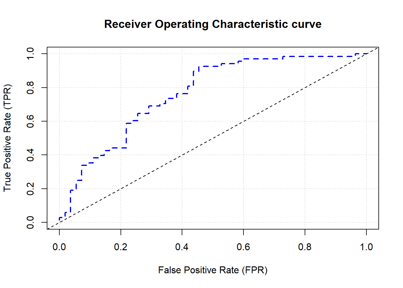
Extracting Accuracy value
accuracy <- h2o.accuracy(performance, thresholds = optimal_threshold)
accuracy
[[1]]
[1] 0.7560976F-measure
f1 <- h2o.F1(performance, thresholds = optimal_threshold)
f1
[[1]]
[1] 0.8076923Sensitivity
h2o.sensitivity(performance,thresholds = optimal_threshold)[[1]]
[1] 0.9264706- Specificity
h2o.specificity(performance, thresholds = optimal_threshold)[[1]]
[1] 0.5454545Error rate
error_rate <- 1 - accuracy[[1]]
error_rate
[1] 0.2439024To explore more on performance measures,Just see the documentation for H2O Model Metric Accessor Functions using ?h2o.metric to see more options regarding the performance measures.
- Saving our best model, we can save the model to load it in future without need to run it again.
model_path <- h2o.saveModel(best_model, path = "models/", force = TRUE)


#to check the model location.
print(paste("Model saved to:", model_path))- To load the saved model, we need to specify the model name, in this case the model name is
GBM_grid_1_AutoML_2_20241023_144643_model_1
saved_model <- h2o.loadModel("models/GBM_grid_1_AutoML_2_20241023_144643_model_1")we can continue to do prediction using new dataset based on the loaded model.
- After completing our predictions and evaluations, shut down the H2O cluster.
h2o.shutdown()Are you sure you want to shutdown the H2O instance running at http://localhost:54321/ (Y/N)? This structured approach outlines the key steps in using H2O AutoML for model training and evaluation. By automating model selection, hyperparameter tuning, and validation, AutoML simplifies the process of building machine learning models, allowing for efficient and robust predictions with minimal manual efforts.
To conlcude, H2O AutoML provides a powerful and user-friendly approach to model training and prediction in R. It simplifies the machine learning workflow by automating model selection, hyperparameter tuning, and performance evaluation across various algorithms. This makes it ideal for users with different levels of expertise, allowing even beginners to generate high-quality model quickly.
By following the steps outlined, we can leverage AutoML to efficiently build, asses, and deploy predictive models without needing deep knowledge of each algorithm. The ability to automate these tasks significantly reduces the time and effort required for model development, making it an essential tool in the machine learning toolkit.
Whether for research, teaching, or practical applications, H2O AutoML streamlines the process of finding the best model, making data-driven decisions more accessible and impactful.